Article - Physically Based Rendering

Introduction

The pursuit of realism is pushing rendering technology towards a detailed simulation of how light works and interacts with objects. Physically based rendering is a catch all term for any technique that tries to achieve photorealism via physical simulation of light.

Currently the best model to simulate light is captured by an equation known as the rendering equation. The rendering equation tries to describe how a "unit" of light is obtained given all the incoming light that interacts with a specific point of a given scene. We will see the details and introduce the correct terminology in a moment. It's important to notice that we won't try to solve the full rendering equation, instead we will use the following simplified version:

To understand this equation we first need to understand how the light works, and then, we will need to agree on some common terms. To give you a rough idea of what the formula means, in simple terms, we could say that the formula describes the colour of a pixel given all the incoming 'coloured light' and a function that tells us how to mix them.

Physics terms

If we want to properly understand the rendering equation we need to capture the meaning of some physical quantities; the most important of these quantities is called radiance (represented with \(L\) in the formula). 
Radiance is a tricky thing to understand, as it is a combination of other physics quantities, therefore, before formally define it, we will introduce a few other quantities.

Radiant Flux: The radiant flux is the measure of the total amount of energy, emitted by a light source, expressed in Watts. We will represent the flux with the Greek letter \(\Phi\). 
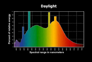
Any light source emits energy, and the amount of emitted energy is function of the wavelength. 

Figure 1: Daylight spectral distribution

In figure 1 we can see the spectral distribution for day light; the radiant flux is the area of the function (to be exact, the area is the luminous flux, as the graph is limiting the wavelength to the human visible spectrum). For our purposes we will simplify the radiant flux with an RGB colour, even if this means losing a lot of information. 

Solid angle: It's a way to measure how large an object appears to an observer looking from a point. To do this we project the silhouette of the object onto the surface of a unit sphere centred in the point we are observing from. The area of the shape we have obtained is the solid angle. In Figure 2 you can see the solid angle \(\omega\) as a projection of the light blue polygon on the unit sphere.

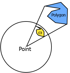Figure 2: Solid angle

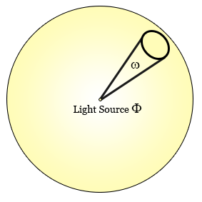
Radiant Intensity: is the amount of flux per solid angle. If you have a light source that emits in all directions, how much of that light (flux) is actually going towards a specific direction? Intensity is the way to answer to that, it's the amount of flux that is going in one direction passing through a defined solid angle. The formula that describes it is \( I =\frac{d\Phi}{ d\omega} \), where \(\Phi\) is the radiant flux and \(\omega\) is the solid angle.

Figure 3: Light intensity

Radiance: finally, we get to radiance. Radiance formula is:

\[L=\frac{d\phi^2}{ dA d\omega cos\theta} \]

where \(\Phi\) is the radiant flux, \(A\) is the area affected by the light, \(\omega\) is the solid angle where the light is passing through and \(cos\theta\) is a scaling factor that "fades" the light with the angle. 

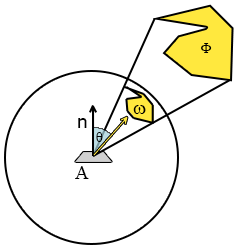Figure 4: Radiance components

We like this formula because it contains all the physical components we are interested in, and we can use it to describe a single "ray" of light. In fact we can use radiance to describe the amount of flux, passing through an infinitely small solid angle, hitting an infinitely small area, and that describes the behaviour of a light ray. So when we talk about radiance we talk about some amount of light going in some direction to some area.
When we shade a point we are interested in all the incoming light into that point, that is the sum of all the radiance that hit a hemisphere centred on the point itself; the name for this entity is irradiance. Irradiance and radiance are our main physical quantities, and we will work on both of them to achieve our physically based rendering.

The rendering equation

We can now go back on the rendering equation and try to fully understand it.

The answer for our second problem, how to solve the integral, is a bit more tricky, because in some cases, we won't be able to solve it quickly enough. But if the BRDF happens to depend only on the incoming radiance, or even better, on nothing (if it's constant), then we can do some nice optimization. So let's see how this happens if we plug in Lambert's BRDF, which is a constant factor (all the incoming radiance contributes to the outgoing ray after being scaled by a constant).

Lambert

Lambert's BRDF sets \(f_r(p,\omega_i,\omega_o) = \frac{c}{ \pi } \) where \(c\) is the surface colour. If we plug this into the rendering equation we get:

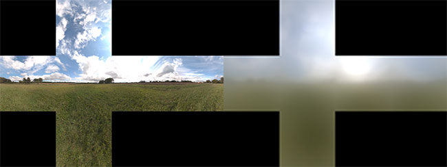Figure 5: Left the radiance map, right the irradiance map (Lambert rendering equation)

Now let's present the shader's code. Please note that for simplicity I'm not using the Monte Carlo integration but I've simply discretized the integral. Given infinite samples it wouldn't make any difference, but in a real case it will introduce more banding than Monte Carlo. In my tests it was good enough given that I've dropped the resolution of the cubemap to a 32x32 per face, but it's worth bearing this in mind if you want to experiment with it.

...
float4 PixelShaderFunction(VertexShaderOutput input) : COLOR
{
    float3 normal = normalize( float3(input.InterpolatedPosition.xy, 1) );
    if(cubeFace==2)
        normal = normalize( float3(input.InterpolatedPosition.x,  1, -input.InterpolatedPosition.y) );
    else if(cubeFace==3)
        normal = normalize( float3(input.InterpolatedPosition.x, -1,  input.InterpolatedPosition.y) );
    else if(cubeFace==0)
        normal = normalize( float3(  1, input.InterpolatedPosition.y,-input.InterpolatedPosition.x) );
    else if(cubeFace==1)
        normal = normalize( float3( -1, input.InterpolatedPosition.y, input.InterpolatedPosition.x) );
    else if(cubeFace==5)
        normal = normalize( float3(-input.InterpolatedPosition.x, input.InterpolatedPosition.y, -1) );

    float3 up = float3(0,1,0);
    float3 right = normalize(cross(up,normal));
    up = cross(normal,right);

    float3 sampledColour = float3(0,0,0);
    float index = 0;
    for(float phi = 0; phi < 6.283; phi += 0.025)
    {
        for(float theta = 0; theta < 1.57; theta += 0.1)
        {
            float3 temp = cos(phi) * right + sin(phi) * up;
            float3 sampleVector = cos(theta) * normal + sin(theta) * temp;
            sampledColour += texCUBE( diffuseCubemap_Sampler, sampleVector ).rgb * 
                                      cos(theta) * sin(theta);
            index ++;
        }
    }

    return float4( PI * sampledColour / index), 1 );
}
...

...
float4 PixelShaderFunction(VertexShaderOutput input) : COLOR
{
    float3 irradiance= texCUBE(irradianceCubemap_Sampler, input.SampleDir).rgb;
    float3 diffuse = materialColour * irradiance;
    return float4( diffuse , 1); 
}
...