Article - World, View and Projection Transformation Matrices

Introduction

In this article we will try to understand in details one of the core mechanics of any 3D engine, the chain of matrix transformations that allows to represent a 3D object on a 2D monitor. We will try to enter into the details of how the matrices are constructed and why, so this article is not meant for absolute beginners. I will assume general knowledge of vectors math and matrices math.

We will first talk about the relationship between transformations and vector spaces. Then we will show how a transformation can be represented in matrix form. From there we will show the typical sequence of transformations that you will need to apply, which is from Model to World Space, then to Camera and then Projection.

Vector Spaces: Model Space and World Space

A vector space is a mathematical structure that is defined by a given number of linearly independent vectors, also called base vectors (for example in Figure 1 there are three base vectors); the number of linearly independent vectors defines the size of the vector space, therefore a 3D space has three base vectors, while a 2D space would have two. These base vectors can be scaled and added toghether to obtain all the other vectors in the space. Vector spaces is quite a broad topic, and it's not the goal of this article to explain them in detail, all we need to know for our purposes is that our models live in one specific vector space, which goes under the name of Model Space and it's represented with the canonical 3D coordinates system (Figure 1). When an artist authors a 3D model he creates all the vertices and faces relatively to the 3D coordinate system of the tool he is working in, which is the Model Space. All the vertices are relative to the origin of the Model Space, so if we have a point at coordinates (1,1,1) in Model Space, we know exactly where it is (Figure 2). Every model in the game lives in its own Model Space and if you want them to be in any spatial relation (like if you want to put a teapot over a table) you need to transform them into a common space (which is what is often called World Space).

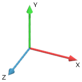Figure 1:Standard Right Handed 3D Coordinate System

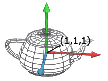Figure 2:Vertex of the teapot in position (1,1,1)

Let me stress this again. It's important to understand that a vector only makes sense within a coordinate system; if we don't specify the space we can't represent any point. Once the model is exported from the tool to the game engine, all the vertices are represented in Model Space. Now, if we want to put the object we just imported in the game world, we will need to move it and/or rotate it to the desired position, and this will put the object into World Space. Moving, rotating or scaling an object it's what we call a transformation. When all the objects have been transformed into a common space (the World Space) their vertices will be relative to the World Space itself.

Transformation

We can see transformations in a vector space simply as a change from one space to another. This is one of the trickiest bits of vector transformations, so let's try to make it as clear as possible.
We can imagine a vector space in 3d as three orthogonal axis (as in Figure 1). We always need to have an "active" space, which is the space that we are using as a reference for everything else (either geometry or other spaces). If we have two models, each one in its own Model Space, we can't draw them both until we define a common "active" space. 
Now let's say that we start with an active space, call it Space A, that contains a teapot. We now want to apply a transformation that moves everything in Space A into a new position; but if we move Space A we then need to define a new "active" space to represent the transformed Space A. Let's call the new active space Space B (Figure 3). Before the transformation, any point described in Space A, was relative to the origin of that space (as described in Figure 3 on the left). After we have applied the transformation all the points are now relative to the new active space, Space B (Figure 3, right). Any operation that re-defines Space A relatively to Space B is a transformation. Notice how, after the transformation, Space A is now "lost" into Space B, or more precisely it's re-mapped into Space B, so we have no way to apply any other transformations to it (unless we undo the transformation and make Space A the 'active' space again).

Another way of seeing this is, imagine that anything in a space moves with the base vectors, and imagine that Space A starts perfectly overlapped over Space B. When we apply the transformation we move Space A away from Space B, and anything in Space A moves with it. Once we have moved all the vertices we then represent all of them as relative to Space B, and we have completed the transformation.

In case we need to operate in Space A again it's possible to apply the inverse of the transformation to Space B. Doing so Space B will be re-mapped into Space A again (and at this point, we "lose" Space B). If we know both transformations and their inverse we can always re-map the two spaces one to the other.

Figure 3: Space Transformations

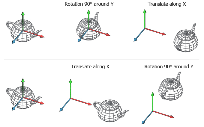
The transformations that we can use in vector spaces are scale, translation and rotation. It's important to notice that every transformation is always relative to the origin, which makes the order we use to apply the transformations themselves very important. If we rotate 90° left and then translate we obtain something very different to what we get if we first translate and then rotate 90° (Figure 4, I've omitted any space apart from the active one).

Figure 4:Different results from same transformations applied in a different order

Figure 4 can also help us understanding the inverse of a transformation a bit more. So if you take Figure 4 top left, the 90° rotation to the left transformation can be removed with it's inverse, which is a 90° rotation to the right. Notice how the inverse of a transformation is a transformation itself, so there is no reason why we shouldn't apply it to objects that are in a completely unrelated space. The inverse of the 90° transformation to the left is a 90° transformation to the right, which obviously can be applied to anything in any space.

Transformation Matrix

Now that we understand that a transformation is a change from one space to another we can get to the math. If we want to represent a transformation from one 3D space to another we will need a 4x4 Matrix. I will assume from here on a column vector notation, as in OpenGL. If you are into row vectors, you just need to transpose the matrix and premultiply the vector where I post multiply it. In order to apply the transformation we have to multiply all the vectors that we want to transform against the transformation matrix. If vectors were in Space A and the transformation was describing a new position of Space A relative to Space B, after the multiplication all the vectors would then be described in Space B.
Now, let's see how we represent a generic transformation in matrix form:

Where Transform_XAxis is the XAxis orientation in the new space, Transform_YAxis is the YAxis orientation in the new space, Transform_ZAxis is the ZAxis orientation in the new space and Translation describes the position where the new space is going to be relatively to the active space. 

Sometimes we want to do simple transformations, like translations or rotations; in these cases we may use the following matrices which are special cases of the generic form we have just presented.

Translation Matrix:

Where translation is a 3D vector that represent the position where we want to move our space to. A translation matrix leaves all the axis rotated exactly as the active space.

Scale Matrix:

Where scale is a 3D vector that represent the scale along each axis. If you read the first column you can see how the new X axis it's still facing the same direction but it's scaled by the scalar scale.x. The same happens to all the other axis as well. Also notice how the translation column is all zeros, which means no translation is required.

Rotation Matrix around X Axis:

Where theta is the angle we want to use for our rotation. Notice how the first column will never change, which is expected since we are rotating around the X axis. Also notice how change theta to 90° remaps the Y axis into the Z axis and the Z axis into -Y axis.

Rotation Matrix around Y Axis:

Rotation Matrix around Z Axis:

The rotation matrices for the Z axis and the Y axis behave in the same way of the X axis matrix.

The matrices I've just presented to you are the most used ones and they are all you need to describe rigid transformations. You can chain several transformations together by multiplying matrices one after the other. The result will be a single matrix that encodes the full transformation. As we have seen in the transformation section, the order that we use to apply transformations is very important. This is mirrored in math by the fact that matrix multiplication is not commutative. Therefore in general Translate x Rotate is different from Rotate x Translate.

Since we are using column vectors we will have to read a chain of transformation right to left, so if we want to rotate 90° to the left around the Y axis, and then translate of 10 units along the Z axis the chain will be [Translate 10 along X]x[RotateY 90°]= [ComposedTransformation].

Let's put some numbers into this so that we can see how it works. Let's say we want to transform the sphere in Figure 5. For simplicity we will apply the transformation only to the top vertex of the sphere which is in position (0,1,0) in Model Space. We will calculate where it's going to be in World Space. First of all we define the transformation matrix. Say that we want the sphere to be placed in the World Space and it will be rotated around the Y axis for 90° clockwise, then rotated 180° around the X axis, and then translated into (1.5, 1, 1.5). This means that the transformation matrix will be:

Please notice how the Result matrix perfectly fits the Generic Transformation formula that we have presented. In World Space the X axis is now oriented as the Z axis of that space therefore it's now (0,0,1). The Y axis is now flipped upside down, hence (0,-1,0). The Z axis is now oriented as the X axis, (1,0,0). Finally, the translation vector (1.5, 1, 1.5).

Once we have the result we can multiply any vertex of the sphere to change it from Model Space into World Space. Let's do our vertex (0,1,0). Notice that since we use a 4x4 matrix we need to use homogeneous coordinates, there fore we need a 4 dimensions vector that has 1 in the last component.

Figure 5:  Sphere transformed from model space to world space

Model Space, World Space, View Space

Now we have all the pieces of the puzzle, let's put them together. The first step when we want to to render a 3D scene is to put all the models in the same space, the World Space. Since every object will be in its own position and orientation in the world, every one has a different Model to World transformation matrix.

Figure 6: Three teapots each one in its own model space

Figure 7: Three teapots set in World Space

With all the objects at the right place we now need to project them to the screen. This is usually done in two steps. The first step moves all the object in another space called the View Space. The second step performs the actual projection using the projection matrix. This last step is a bit different from the others and we will see it in detail in a moment.

Why do we need a View Space? The View Space is an auxiliary space that we use to simplify the math and keep everything elegant and encoded into matrices. The idea is that we need to render to a camera, which implies projecting all the vertices onto the camera screen that can be arbitrarily oriented in space. The math simplifies a lot if we could have the camera centered in the origin and watching down one of the three axis, let's say the Z axis to stick to the convention. So why not to create a space that is doing exaclty this, remapping the World Space so that the camera is in the origin and looks down along the Z axis? This space is the View Space (sometimes called Camera Space) and the transformation we apply moves all the vertices from World Space to View Space.
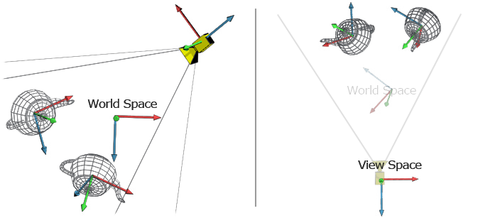
How do we calculate the transformation matrix for View Space? Now, if you imagine you want to put the camera in World Space you would use a transformation matrix that is located where the camera is and is oriented so that the Z axis is looking to the camera target. The inverse of this transformation, if applied to all the objects in World Space, would move the entire world into View Space. Notice that we can combine the two transformations Model To World and World to View into a single transformation Model To View.

Figure 8: On the Left two teapots  and a camera in World Space; On the right everything is transformed into View Space (World Space is represented only to help visualize the transformation)

Projection Space

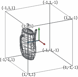
The scene is now in the most friendly space possible for a projection, the View Space. All we have to do now is to project it onto the imaginary screen of the camera. Before flattening the image, we still have to move into another, final space, the Projection Space. This space is a cuboid which dimensions are between -1 and 1 for every axis. This space is very handy for clipping (anything outside the 1:-1 range is outside the camera view area) and simplifies the flattening operation (we just need to drop the z value to get a flat image).
To go from the View Space into the Projection Space we need another matrix, the View to Projection matrix, and the values of this matrix depend on what type of projection we want to perform. The two most used projections are the Orthographic Projection and the Perspective Projection.

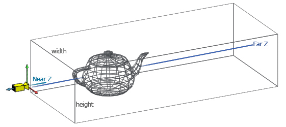
To do the Orthographic projection we have to define the size of the area that the camera can see. This is usually defined with a width and height values for the x and y axis, and a near and far z values for the z axis (Figure 9).

Figure 9: Orthographic Projection

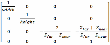
Given these values we can create the transformation matrix that remaps the box area into the cuboid. The matrix that follows is transforms vectors from View Space into Ortho Projected Space and assumes a right handed coordinates system.

Figure 10: Projection Space obtained from the teapot in Figure 9

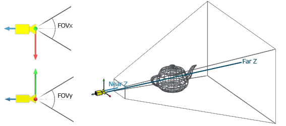
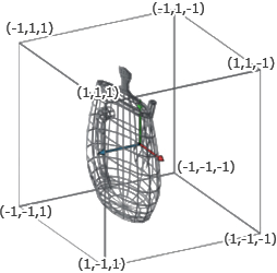
The other projection is the perspective projection. The idea is similar to the orthographic projection, but this time the view area is a frustum and therefore it's a bit more tricky to remap. Unfortunately the matrix multiplication in this case is not enough, because after multiplying by the matrix the result is not on the same projective space (which means that the w component is not 1 for every vertex). To complete the transformation we will need to divide every component of the vector by the w component itself. Current graphics APIs do the division for you, therefore you can simply multiply all your vertices by the perspective projection matrix and send the result to the GPU.

 

 

Figure 11: Perspective Projection

GPU takes care of dividing by w, clipping those vertices outside the cuboid area, flattening the image dropping the z component, re-mapping everything from the -1 to 1 range into the 0 to 1 range and then scale it to the viewport width and height, and rasterizing the triangles to the screen (if you are doing the rasterization on the CPU you will have to take care of these steps yourself). We can therefore take these last steps for granted if we render via OpenGL or DirectX, so the perspective space is the last step of our chain of transformation.

Finally a model can be transformed for rendering chaining [View To Projection]x[World To View]x[Model to World]=[ModelViewProjectionMatrix].